Claims denials: predicting acceptance / denial of claims

In today's post, we develop a predictive model that could be used to predict whether a medical expense claim will be accepted by an insurance company before the claim is made.  In order to do this, we will use the IBM SPSS Modeler data mining workbench to understand underlying relationships in observed data to train the predictive model.  The steps we will follow are as follows:

1) Understanding the data: among other things, this step will include determining which fields in the data to use as predictors and which ones to discard.

2) Partitioning the file: this step can be done within IBM SPSS Modeler by using the Partition node.  However, for today's post, we will do this in excel prior to creating the model.

3) Training the model: we will use one of the partitioned files to train the model.

4) Scoring the model: we will use the other partitioned file to score the model.

Let's get started.

Understanding the data

Since our data is in an excel file, we start with an excel source node and attach the data file to the source node.  On adding a table node, to the file, we observe several fields that should not be used as predictors:

* Rejection Code 1 and Rejection Code 1 Description: we would only know these fields after the fact and so they should not be included as predictors.  Taking these into account would be like predicting if a movie won an Oscar Award by using our actual knowledge of whether that movie had won or not.
* Approved: same reason as above.
* Variance (Expected Amount - Approved): this is a calculated field.  Since we ignore Approved, we have to ignore this field as well.
* Expected Allowed Amount: all records in this field have zero values and so can be ignored.
* Variance (Expected Amount - Approved): this is a calculated field.  All records in this field have zero values and so can be ignored.

We also ignore Payment, Adjustment, Expected Payment, Credit and Debit fields in order to remove the impact of the cost of the procedure as well as mode of payment from the predictive model.  A case could be made for leaving these fields in as predictors but for the purposes of this post, we will ignore them.

Next, we attach a distribution node to the source node to see the distribution of claims across the different calendar periods to see if there is any discernible pattern.

On executing this node, we observe the following results:

While there are some months that have a greater number of claims than others, there is no clear seasonal pattern that emerges.  Consequently, we ignore Calendar Period, Calendar Quarter and Calendar Year.

We also attach a distribution node to the source node to check the distribution of the denial category and observe the following values:

The records with "$null$" represent claims that have been Approved.  From this chart, we observe that approximately 70% of the claims have been approved.  Of the rejected claims, approximately 50% are due to "No Prior Authorization Adjustment" and the remaining 50% are split across 13 different causes / reasons.

At the outset, our objective is to simply predict which claims will be Approved and which ones will be Rejected.  Therefore, while training the model, we will reclassify the Denial Category fields into two Categories:

* All records with "$null$" will be reclassified as Approved
* All other records will be reclassified as Denied.

Partitioning the file

The original data file contains 10,535 records.  In our next step, we partition the original file into two separate files:

1) Training data set the includes the first 10,000 records; and
2) Scoring data set that includes the last 535 records.

Training the model

Once again, we start with an excel source node and attach the training data set that includes the first 10,000 records to this node.  We then attach a Filler node in order to change the $null$ values in the Denial Category field to "APPROVED".  This is done as follows:

We then attach a table node to see the results of our actions:

As can be seen from the table above, the $null$ values in the Denials Category field have been replaced by APPROVED.

We then attach a filter node to remove the following fields:

We then attach a derive node to create a new field "New Denial Category" that only contains the values APPROVED and DENIED as follows:

A table contained the new field is provided below:

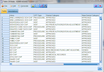
We then attach a type node to identify our target filed as follows:

As can be seen from the table above, the New Denial Category field has been classified as the Target.  Since the New Denial Category field is derived from the Denial Category field, we set the value of that field to None to ensure that it does not play a role in predicting the New Denial Category field.

We then attach a C5.0 modeling node and run the model with default options.  In order to evaluate the accuracy of the predictive model, we attach an analysis node to the modeling nugget.  We observe the following results:

As can be seen from the table above, the model predicts denials with almost 96% accuracy!  We browse the model nugget to obtain further insight into the predictor importance and we observe the following:

The decision tree generated by IBM SPSS Modeler is as follows:

The completed modeling stream is as follows:

Scoring the model

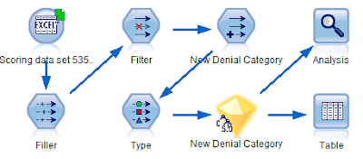
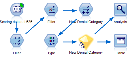
In order to score the model, we use the scoring data set consisting of 535 records.  Since this file is also in excel format, we attach it to an excel source node.  We then attach the modeling nugget to the excel source node as follows:

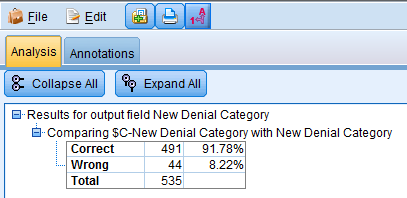
On running the analysis node, we see the following results:

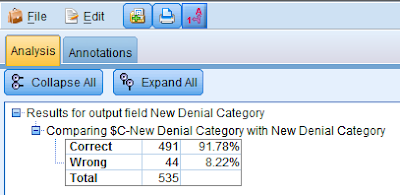
The analysis node compares the values in the New Denial Category (observed values) with values in the field $C-New Denial Category (predicted values).  As can be seen the model accurately predicted 491 records of a total of 535 records giving us an accuracy rate of approximately 92%.