Market Basket Analysis
Affinity analysis is a data analysis and data mining technique that discovers co-occurrence relationships among activities performed by (or recorded about) specific individuals or groups. In general, this can be applied to any process where agents can be uniquely identified and information about their activities can be recorded. In retail, affinity analysis is used to perform market basket analysis, in which retailers seek to understand the purchase behavior of customers. This information can then be used for purposes of cross-selling and up-selling, in addition to influencing sales promotions, loyalty programs, store design, and discount plans [Source: Wikipedia].
In today's post, we use fictitious data from a supermarket describing items bought together by a set a individuals along with personal data that can be acquired through a loyalty scheme. We will use SPSS Modeler to identify relationships between items bought together so we can understand which items are typically bought together and the profile of shoppers that typically shop for these items. This information is valuable because as mentioned above, it can used by the supermarket to create promotions, improve customer satisfaction and increase revenue.
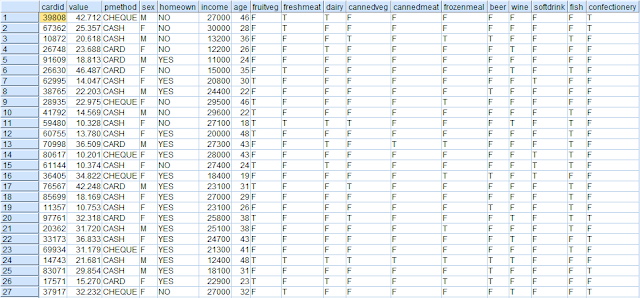
We start with the data which contains the following fields:
CardId: refers to the loyalty scheme ID of each customer
Value: refers to the amount that they spent during a visit to the store
Pmmethod: refers to the method of payment
Sex, income, homeown and age provide further descriptive information about the shoppers
The remaining fields indicate what these shopper purchased. For example, if a shopper purchased Fish, the flag T is used to indicate this.
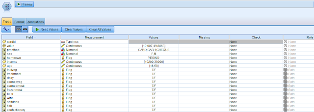
The first step in our analysis is to determine whether or not a pattern even exists between the various items that are purchased in the supermarket. In order to do this, we first add a type node and change the role of all fields except the items purchased to None. The roles of the items purchased are set to Both (i.e. both Input and Target) as follows:
We then add an Apriori node to the type node and execute the node. A priori means "from the earlier" and is used in philosophy to mean knowledge or justification that is independent from experience, e.g. all bachelors are unmarried [Source: Wikipedia]. In computer science and data mining, Apriori is a classic algorithm for learning association rules. Apriori is designed to operate on databases containing transactions (for example, collections of items bought by customers, or details of a website frequentation). As is common in association rule mining, given a set of item sets (for instance, sets of retail transactions, each listing individual items purchased), the algorithm attempts to find subsets which are common to at least a minimum number of the item sets. Apriori uses a "bottom up" approach, where frequent subsets are extended one item at a time (a step known as candidate generation), and groups of candidates are tested against the data. The algorithm terminates when no further successful extensions are found [Source: Wikipedia].
On reviewing the results of the Apriori algorithm, we observe the following:
As can be seen from the table above, where a customer buys beer and cannedveg, they are also likely to buy a frozenmeal and so on. Support % refers to the number of times that this trend is spotted in the data and the confidence % refers to likelihood with which this sequence of events will occur. In order to get a better understanding of the relationships between different items purchased, we attach a web node and see the following:
As can be seen from the web chart above, there are three distinct associations that come to light:
1) Fish and fruitveg - let us call this category "Healthy".
2) Confectionery and wine - let us call this category "Wine_Chocs".
3) Beer, frozenmeal and cannedveg - let us call this category "Beer_Beans_Pizza".
We use the web chart to create new fields in our data for each of these associations as follows:
1) If Fish = T and if Fruitveg = T, then Healthy
2) If Confectionery = T and if Wine = T, then Wine_Chocs
3) If Beer = T, Frozenmeal = T and if Cannedveg = T, then Beer_Beans_Pizza
We then add a C5 rule induction algorithm node to each of these categories to determine the profile of the shoppers that belong to each of these categories. For more information on the C5 algorithm, see here. In order to do this, we treat all the descriptive variables as Inputs, the category we are trying to define as a Target and all other variables as None. For example, the type node for the Healthy analysis appears as follows:
By executing the C5 algorithm, we observe the following results:
Healthy:
The most important predictors of the Healthy category are as follows:
The decision tree generated for determining the Healthy category is as follows:
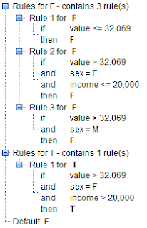
From this decision tree, we observe the following rules for identifying the Healthy category (by clicking on Generate --> Rule Set):
From our analysis, it appears that the only Healthy eaters are those below the age of 24 years old who do not own their own homes.
Wine_Chocs
The most important predictors of the Wine_Chocs category are as follows:
The decision tree generated for determining the Wine_Chocs category is as follows:
From this decision tree, we observe the following rules for identifying the Wine_Chocs category:
Beer_Beans_Pizza
The most important predictors of the Beer_Beans_Pizza category are as follows:
The decision tree generated for determining the
Beer_Beans_Pizza category is as follows:
From this decision tree, we observe the following rules for identifying the Beer_Beans_Pizza category:
From the rule set, we can see a clear demographic profile for this group: men with an income of less than or equal to 16,900.
This type of profiling can be extremely useful to target special offers to improve response rates of direct mail campaigns or in retail assortment planning where a stores inventory can be matched to the demands of its demographic base.


Comments
Post a Comment