Introduction to the K-Nearest Neighbor (KNN) algorithm
In pattern recognition, the K-Nearest Neighbor algorithm
(KNN) is a method for classifying objects based on the closest training examples
in the feature space. KNN is a type of instance-based learning, or lazy
learning where the function is only approximated locally and all computation is
deferred until classification. The KNN algorithm is amongst the
simplest of all machine learning algorithms: an object is classified by a
majority vote of its neighbors, with the object being assigned to the class
most common amongst its k nearest neighbors (k is a positive integer, typically
small). If k = 1, then the object is simply assigned to the class of its
nearest neighbor [Source: Wikipedia].
In today's post, we explore the application of KNN to an automobile manufacturer that has developed prototypes for two new vehicles, a car and a truck. Before introducing the new models into its range, the manufacturer wants to determine which of the existing models in the marketplace are most like the prototypes. In order words, which of the existing vehicles in the market place are the "nearest neighbors" to the prototypes and therefore which vehicles are the prototypes most likely to compete against. Needless to say, this information would be a crucial input to the marketing strategy of these two prototypes.
As always, we first start with the data which is as follows:

As can be seen, this data file contains 16 fields (variables) and 159 records. The variables include information like type (0 = sedan; 1 = truck), price (sale price in thousands), engine size, horsepower, mpg, etc. The last two rows (158 and 159) in the data file refer to the prototypes developed by the manufacturer:

The last field (or column or variable) in the data file is called "Partition". This field has values of "0" for all records in the data file except the last two rows. This serves as a "flag" field so that we only consider the existing automobiles in the marketplace as inputs in our analysis (since we want to classify our prototypes, it does make sense to treat them as inputs in our analysis).
We will use SPSS Modeler v 15 for our analysis. To get started, we attach a Type node to the data file. Since we want to classify our prototypes based on features, we treat all fields from "Price" through "Mpg" as inputs in our analysis. We also treat the "Partition" field as an input for the reason discussed above. All other fields are treated as "None". The completed type node, appears as follows:

Next, we attach a KNN Modeling node to the Type node and choose the following options:
1) Only identify the nearest neighbors
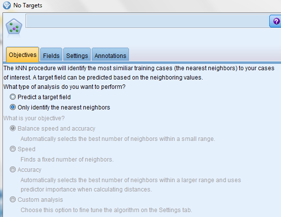
2) Identify the focal record using the Partition field:

Upon executing the node, we obtain the following results:

This chart classifies our prototypes (in red) based on their nearest neighbors in accordance with three predictor variables: engine size, price in thousands and horsepower. This is a 3D interactive chart that identifies the 3 nearest neighbors (K = 3) to our prototypes. The next chart, called the Peers chart, displays our prototypes along with their nearest neighbors across all six input fields as follows:

From this chart, we can tell that one of our prototypes has the lowest engine size (158) whereas our other prototype (159) has the largest engine size when compared to the existing automobiles in the marketplace. Similar conclusions can be drawn on reviewing the other six inputs. For example, 158 has the lowest horsepower and 159 has the largest width.
Next we review the k Nearest Neighbors and Distances chart:

This chart tells us that the nearest neighbors for 158 are:
- 131: Saturn SC;
- 130: Saturn SL; and
- 58: Honda Civic.
Similarly, the nearest neighbors for 159 are:
- 105: Nissan Quest;
- 92: Mercury Villager; and
- 101: Mercedes Benz M-Class.
Upon comparing our prototypes with their nearest neighbors based on four criteria (price, engine size, horsepower and mpg), we obtain the following results:

From this table, we can clearly see that the main advantage the prototypes have over their nearest neighbors is in the "mpg" area: the prototypes are far more fuel efficient than their nearest neighbors. The marketing message would therefore have to focus on this benefit when these prototypes are launched.


Pretty good post. I just stumbled upon your blog and wanted to say that I have really enjoyed reading your blog posts. Any way I’ll be subscribing to your feed and I hope you post again soon.
ReplyDelete360DigiTMG